Checklists and Conditional formatting for task management

Welcome! If you are new to this blog; the sit you're in is yours. If you want to keep it, please subscribe. If you are already subscribed, then I am glad to have you back. Let's be friends forever.

I'm a sucker for simple English! This is why I find writing so difficult—I want to talk about conditional formatting without using big words like "conditional" ad "formatting" but I also need to finish this post before my next wave of procrastination hits.

So, let's do this! What is conditional formatting? Conditional formatting is a way to change the appearance of your information based on a rule you set. In spreadsheets, conditional formatting changes the appearance of cells based on the values in the cells and the condition(s) set for those values. For example: everyone with a score below the pass mark can be highlighted in red.

Conditional formatting has several uses and I want to show you at least one today. I will use our friend Yücel's example to show you how to create checklists and manage tasks in a Google spreadsheet.

Creating checklists to track tasks in Google Sheets

Yücel uses Google Workspace for all project management for Big Sleep Arts (If you don't know Yücel, that's what happens when you skip class—Read this). This time round, Yücel wants the sales team to complete certain tasks by Friday this week and he uses a Google spreadsheet to track the progress of the tasks. Fire up your Google spreadsheet and live vicariously through this artist since your parents forced you to do engineering or medicine instead (take a second if this is a trigger for you). Here is what the spreadsheet looks like initially:

Sales team tasks

Adding checkboxes

Yücel wants to add checkboxes in the Done column because the basic life is not their portion. To add checkboxes in the Done column, Yücel clicks in the first cell in the column (B2), goes to Insert on the toolbar and clicks Checkbox.

Inserting a checkbox

A checkbox is added to cell B2

A checkbox in B2

Yücel notices that when the checkbox is unchecked, its value is FALSE as seen in the Formula bar below.

And when the checkbox is checked, its value in the formula bar is TRUE, which would correspond to a completed task in this case. The knowledge of the value of the checkbox (TRUE or FALSE) when checked or otherwise will be useful soon (put a pin in this).

Yücel then copies the checkboxes downwards to all the other relevant cells in the Done column (B2:B9) by clicking in cell B2 and then hovering the cursor over the bottom right corner of the cell until the cursor turns into a black cross. Once the black cross is visible, Yücel clicks, holds and drags downwards from cell B2 to B9. Cells B2:B9 all have checkboxes now.

Checkboxes copied from cells B2 to B9

Using conditional formatting

The guy outside has decided to mow the lawn before 9AM, so Yücel is furious but alert. Yücel channels his anger into productivity by using conditional formatting to change the appearance of (or format) the cells in the Tasks column when a task is marked Done by checking the box in the corresponding adjacent cell. To format the tasks, Yücel selects all the relevant cells in the Tasks column (A2:A9). While the cells are selected, they go up to the tool bar, under Format, and select Conditional Formatting

Select range and click Conditional formatting

The conditional format rules tab opens up on the extreme right side of the window and Yücel selects Single Color instead of Color Scale.

In the Conditional format rules open tab, we check to ensure we are formatting the range we want. Under Apply to range, we see A2:A9, which is our desired range for formatting. The range should be correct by default since Yücel selected the right range of cells before clicking Conditional formatting.

Double check the range

Changing the appearance or formatting

Yücel wants the completed tasks to be blurred and crossed out with a straight line through them when a checkbox is checked. Let's see how Yücel does this.

Step 1.

In the Conditional format rule tab, under Format rules, in the dropdown called Format cells if..., select Custom Formula is. Below Custom Formula is, there is a provision to enter a Value or Formula. Enter this formula: =B2=TRUE (Just do and ask questions later).

Add a Custom Formula as a format rule

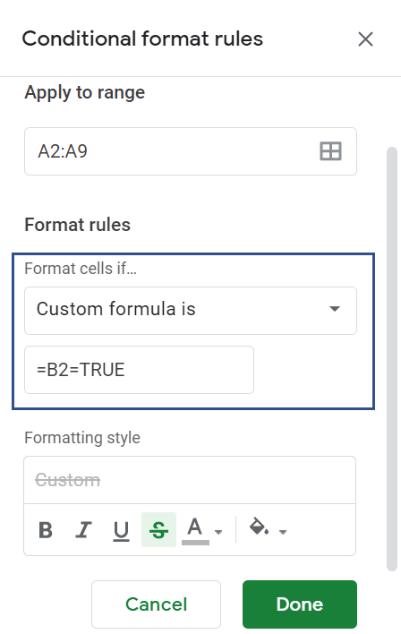
Step 2.

Below the box where the formula is entered are the Formatting style options. The formatting style options change the appearance of the values in our desired range (A2:A9) in real time when the condition in the formula is met. For the formatting style, Yücel blurs the completed tasks by changing the font color to grey and crosses the tasks out by selecting "Strikethrough". The fill color is left as white (because one needs to know one's limits). The formatting style is previewed in the box below Formatting style and once Yücel likes the preview, they click Done.

Formatting styles

Explaining the formula (=B2=TRUE)

Ok, you can lower your hands now, you keeners. What does our formula (=B2=TRUE) mean? Where do we get it from? Let's break it down:

1. The Equal sign: Every time we type a formula in Google Sheets or Excel, we must start with an equal sign (=).

2. The B2: The range we want to format is the Tasks column (A2:A9), and we want the format to change when the corresponding checkboxes in the Done column (B2:B9) change (checked or unchecked). Writing B2 tells Google Sheets to look inside the first cell in the Done column (which corresponds to the first task in the Task column (A2)) and check the appearance of the checkbox. Google Sheets is smart and keeps matching the tasks with their corresponding checkboxes in the Done column. Starting with B2 simply provides initial guidance and Google Sheets does the rest. Therefore, when Yücel moves to another task in the Tasks column—say from A2 to A3—the task in A3 now corresponds to the value in B3.

3. The "=TRUE": Remember when Yücel noticed that when the checkbox is unchecked, its value is FALSE and when the checkbox is checked, its value is TRUE? It is game-time. The "=TRUE" refers to a checked checkbox and allows us to tell Google Sheets to format the tasks only when they are marked as done like so:

Checked box equals formatted task

Putting it all together, since Yücel wants to change the appearance of the completed tasks, Yücel selects the range of tasks and tells Google Sheets: "For each task in my column of Tasks (A2:A9), whenever you see a checked box (whose value is TRUE) in column B next to the task, change the appearance of the task based on the formatting style I choose."

Final product

Yücel looks at the previewed formatting style and is satisfied. They check to see if the formatting is working as planned by checking some of the checkboxes. The result is shown below.

Checked boxes change the appearance of tasks

Practical application

Yücel is almost done! The checklist is pretty and all but this feature is more useful if Yücel's team can collaborate with him in the spreadsheet. For this, Yücel assigns the tasks to the Person responsible, by tagging them using their email address. To tag the person, they click in the cell containing the person responsible (Jane in the example below), right click and select Comment.

Assigning a task to Jane by adding a comment

After clicking Comment, a dialogue box opens where Yücel can type a passive aggressive message to Jane, laden with several "please kindly"-s. To tag Jane so she gets an email alert when the task is assigned, Yücel types a plus (+) (or the @) sign in front of Jane's email address in the dialogue box and checks the box that says "Assign to [Jane's email]".

Assignment of tasks to Jane

Bonus feature

One of the employees, Tuna, bless their heart, loved Yücel's creation and wanted to show off the skills they learned from a certain online blog they subscribe to (hint hint). Tuna suggests Yücel adds another column for only outstanding tasks instead of having them combined in the same column with the completed tasks. Tuna uses the FILTER function for this:

The FILTER function takes the following arguments: the range to filter and the condition(s) used to filter the range.

Arguments for FILTER function

The range to filter is our Tasks column (A2:A). The condition is if the cells in the Done column are FALSE (B2:B=FALSE). Remember FALSE means undone or outstanding. To ensure the formatting applies as tasks are added, Tuna selects the entire columns instead of using A2: A9 and B2:B9 respectively.

FILTER function in action

Once Tuna closes the bracket of the FILTER function and presses Enter, a dynamic list of the outstanding tasks is created. This list updates automatically as tasks are completed or reopened.

Outstanding tasks update automatically

Conclusion

Conditional formatting can be a game-changer for presenting information creatively. From flagging low sales in certain months, and low scores in exams to highlighting completed tasks, the options are endless on the condition (see what I did there?) that you know exactly what you want to accomplish.

PS: If you have any questions, comments or concerns about any of the concepts I have tackled in this article, OR if you know better tricks, please reach out to me. I would love to hear from you. Otherwise, please subscribe to this blog for more updates.

Subscribe for more posts like this